Jim Bolton, Ph.D., president, Bolton Photosciences, Inc.
In 2006, the US Environmental Protection Agency (USEPA) issued the Long Term 2 Enhanced Surface Water Treatment Rules (LT2ESWTR) (USEPA 2006) and the Ultraviolet (UV) Disinfection Guidance Manual (UVDGM) (USEPA 2006b).
In 2020, the USEPA issued an additional guidance document titled “Innovative Approaches for Validation of Ultraviolet Disinfection Reactors for Drinking Water Systems” (Innovative Approaches) (USEPA 2020). These documents serve as the basis for regulating UV disinfection treatment in drinking water treatment plants throughout the US and many other parts of the world.
The regulations are based on specifying minimum UV doses (given in the LT2ESWTR) for the inactivation of Cryptosporidium, Giardia and other viruses. The guidance manuals (UVDGM and Innovative Approaches) then specify how a UV disinfection reactor must be validated by biodosimetry to deliver the minimum UV doses.
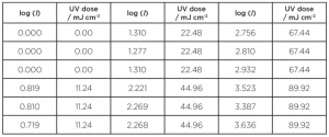
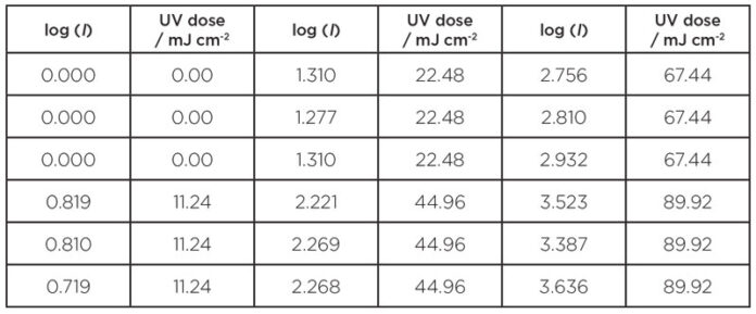
In the “calculated dose approach,” the biodosimetry process involves challenging the UV reactor with a surrogate microorganism (usually MS2 coliphage) and determining the log inactivation [log(I) = log(N0/N), where N0 is the number of viable microorganisms in the influent and N is the number in the effluent)] for a matrix of ultraviolet transmittance (UVT) and flow rates. At the same time, a sample of the influent water is subjected to a collimated beam test where the UV dose-response curve is determined for the challenge microorganism (e.g., MS2), which consists of a series of experimental log reductions for a range of UV doses. Table 1 gives an example of the data for a typical UV dose-response curve.
At this point, one must determine the independent and dependent variables. To make this choice, one must realize that the statistics that are used to analyze a set of x, y data are based on the assumption that one set of variables is essentially error free and the other set of variables carries almost all of the experimental error.
In this case, clearly the UV dose is the most accurate. Thus it is logical to assume that the UV dose is the independent variable (usually designated as x), thus the log (I) becomes the dependent variable (usually designated as y).
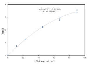
The next step is to choose a fitting function for a regression analysis. In this case, it appears that a quadratic function forced through zero is best. Figure 1 shows a plot of the log (I) vs. UV dose and the fitted regression function.
The procedure for the determination of the Reduction Equivalent Dose (RED) involves calculating the log (I) from each pair of influent and effluent samples in the flow-through UV rector tests. Each log (I) then must be matched against the UV dose-response curve from the collimated beam tests (Figure 1).
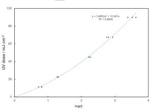
The UVDGM and the Innovative Approaches guidance documents each recommend the collimated beam data (Table 1) be plotted as UV dose vs. log (I) (Figure 2).
The regression equation then can be used to obtain UV doses for each log (I) from the flow-through results. However, there is a problem with this approach. As seen in Figure 2, the errors are in the log (I) variable. Thus, it is not valid to carry out a regression analysis in this manner.
One must realize there is only one valid regression analysis that will satisfy the error requirements for the selection of the independent and dependent variables. Returning to Figure 1, the unique quadratic fit equation can be rearranged from
log(I) = ax2 + bx (1a)
to
ax2 + bx – log(I) = 0 (1b)
where x = UV dose.
The solution to Equation 1b is
(1c) 
Alternatively, one could compute log(I) from Equation 1 for a wide range of closely spaced x values and estimate log(I) for a given x value by linear interpolation.
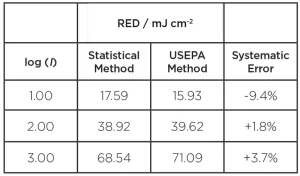
To illustrate the systematic errors that are introduced by using the (incorrect) USEPA method, Table 2 shows the comparison between the two methods, that is:
Proper statistical method – obtain log(I) values from Equation 1c or from a table of UV doses vs. log(I)
USEPA method – plot UV dose vs. log(I), and use the new regression equation to derive UV doses (REDs) for given log(I) values
Note that a negative error is conservative in that the USEPA method would underestimate the RED. The percent errors in Table 2 would carry through to the calculation of the validated UV dose.
Note also that this example is a specific data set for MS2. The errors may be quite different for other data sets and other microorganisms.
The systematic errors shown in Table 2 are significant. It is true that these systematic errors are comparable to the random errors found in biodosimetry measurement, but why introduce unnecessary systematic errors arising from an erroneous method?
In conclusion, it is recommended that an addendum be added to the USEPA guidance documents to recommend changes to the method used to estimate the UV dose from collimated beam data.
Contact: Jim Bolton, [email protected]
References
USEPA 2006. Ultraviolet Disinfection Guidance Manual for the Final Long Term 2 Enhanced Surface Water Treatment Rule[Online]. Available: https://nepis.epa.gov/Exe/ZyPDF.cgi?Dockey=600006T3.txt.
USEPA. 2020. Innovative Approaches for Validation of Ultraviolet Disinfection Reactors for Drinking Water Systems. https://cfpub.epa.gov/si/si_public_record_report.cfm?Lab=NRMRL&direntryid=328890

